Visualizing bulk samples with a statistical summarizer

Visualizing bulk samples...

Often there is more data available than is convenient to see at once. For example on a 'scope you can zoom in and out (a bit) of the capture buffer using the horizontal timebase, and move around in the capture buffer within its bounds.

In our case we will usually have a 160 x 128 window to view our data through, but we are generating 8 channels of samples per ms, and storing them in hyperram. Trying to see every sample as 1px, at 6fps we could show each sample once for one frame, and at our actual 30fps each sample would be on-screen for 5 frames, proceeding leftwards at 52px / frame. That should be fine if it's what you want to see.

Since we have room for 4 minutes of capture buffer, and we might care more about an overview of what is happening on a slower scale than every sample flashing by. So we have this same kind of problem of how to render as much useful detail as possible.

Oscilloscopes have had this problem for a while and there are some well-known ways of handling it...

Just undersampling the buffer

Cheap and midrange digital scopes deal with this by just undersampling the signal, ie, to "zoom out" by a factor of ten they just show every tenth sample.

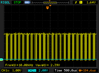
This works, but there is a lot of messy aliasing and lost information; for example some subsamples show as 1px gaps in the blocks of data, but it is misleading: there are no gaps just the subsampling happened to hit a '0'. It's made worse because the scope either sets a pixel to full intensity or not.

Averaging

Even cheap digital scopes offer multi-trigger averaging, which can be useful if your signal capture is synchronized. However it only suits some kinds of problem and requires synchronous capture. For example the mean of an unlocked sine wave is zero: if this was the method for zooming in and out your signal would appear to attenuate and then completely disappear into a flat line as you zoomed out.

Basically it's a good way to reduce unpredictable noise (by attenuating low probability data), but it doesn't do the representation of the time series well. It basically reduces the data set by throwing out devations from the mean.

Digital Persistence

You can use a digital 'scope's 'persistence' setting to retain some number of old samples in the display buffer, this helps to estimate the union of where the signal goes but again pixels are on or off, there's no information about how often a pixel is set, just the extent of what was ever set during the persistence period.

Analogue Persistence

Analogue scopes did a better job in respect of representing the available data as the phosphor on the back of the CRT glass automatically averaged the "hit rate" as intensity levels

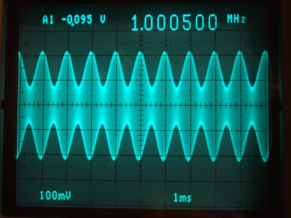(From http://www.tapeheads.net/showthread.php?t=30477)

Expensive digital scopes simulate this digitally

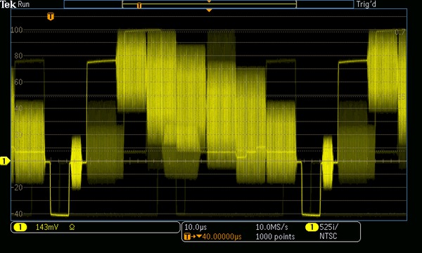(From http://www.tek.com/datasheet/mixed-domain-oscilloscopes-3)

Statistical intensity

In short what is needed is when "compressing" multiple samples into one column of pixels for a time-compressed "zoom out" type view, each pixel in the column should represent the count of that row being lit in the raw samples.

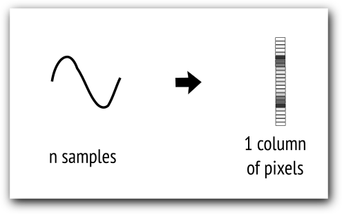
Notice that this is not related to reducing the input to a single number like a mean or even a median; the output may be discontiguous even with multiple regions active if that was what the incoming data set showed.

Dynamic range of accumulator vs display

Every row with samples in the original sample set is represented by accumulating it in a row accumulator array. Once that is done though, the count in the row accumulator, which can exceed 4096 in the integer part, is scaled to be represented by effectively only 32 possible pixel intensities. That means we can't display probabilities below 3% due to the display hardware.

In the worst case, 4096:1 summarization (4s:1px) on 12-bit counts, counts 0 to 127 all map on to pixel intensity level 0, and are indistinguishable from no counts.

For summarization at 32:1 (30ms:1px) and below though, the pixel intensities have enough dynamic range to represent all 32 possible counts.

Vertical antialiasing

A different but related issue is around vertical antiliasing: there are only 128 vertical pixel rows in the display, and at full vertical scale, 0 - 30V, common, smaller voltages < 5V map into just the low 25 pixels (the scale can be changed dynamically to improve this, but still it won't be uncommon to see it on full scale especially if a second channel has higher voltages displayed simultaneously).

It means that under those worst-case conditions, each row on the display is representing around 250mV, which is very coarse. Another problem is that near the limit of the mapping to one line, eg, say, 1.248V, small noise will cause the next vertical line to get more or less hits as well.

The overall quality can get a big improvement by using fractional accumulation on both the current row and the "next" row.

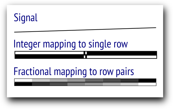
Instead of accumulating a '0' or '1' for a 'hit' on a row in the sample being compressed, the accumulator is changed to hold a 12.4 bit fraction. 15 "fractional points" are shared between the current and next line each time.

If the sample is exactly on the row value, all 15 points go on the current row accumulator and nothing on the next row's accumulator. If it's halfway, 8 and 7 are shared between the rows. In this way, more information about the fractional voltage can be retained as part of the summary accumulation and a more accurate result obtained.

... with a Statistical Summarizer

The statistical summarizer I implemented to do this is a mode of the generic blitter I described before. This allows reuse of the Hyperram FIFOs and blitter descriptor queue conveniently and economically in terms of FPGA space.

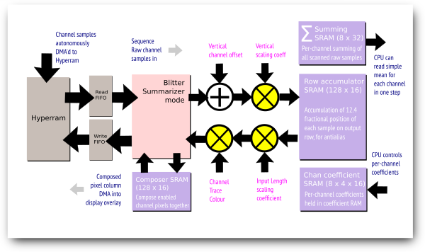
The summarizer mode, range of sample addresses, and where to draw the column of pixels, is fetched from the blitter descriptor.

The summarizer "compresses" sample information for up to 8 channels x 4K samples into a single column of pixels, using the techniques mentioned above.

All of the summarizer operations take place on contiguous samples taken from Hyperram, not at acquisition time. That means the same, fully detailed sample buffer can be rendered at different levels of detail after capture arbitrarily.

Step 1: Acquire raw samples

A dedicated hardware sequencer acquires the set of channel samples at the right time and DMA's them into a ringbuffer per-channel in the Hyperram. Altogether 10 channels are read and 8 stored in the hyperram.

Step 2: For each channel, iterate through the samples to be summarized

A sequencer in the blitter zeros down the row accumulator and composer SRAM, and then for each channel, iterates through the stored sample channel data from Hyperram, scaling it with a dedicated multiplier according to the current vertical display scale and accumulating it in bins corresponding to the vertical output.

This step does the fractional accumulation (12.4 bits) and spreads the result between two adjacent lines according to the fractional part.

Step 3: Translate the hits to the RGB trace colour intensity

The trace colour for the channel is then scaled according to the relative amount of hits accumulated in the bins. This also uses a dedicated multiplier.

Step 4: Compose all the trace RGB data

For each channel, the scaled RGB for the trace is composed into a 1-column SRAM until all the channels have been accounted for.

Step 5: Blit the composed RGB pixels

Then the composed pixels representing all the channel trace renderings is blitted into the framebuffer in Hyperram.

A 32-bit sum of all the samples is also kept and used both for computing a headline mean to be shown numerically, and for computing "area under the curve". Dividing this by the number of samples added gives the mean.

The ICE5 provides four dedicated 16x16 hardware multipliers, three are used here to

scale the sample data (usually 16-bit) to a pixel row. This encapsulates the equivalent of a 'scope "vertical scale" control setting V/div. Actually the row mapping is fractional, 4 fractional bits are used to modulate the value accumulated in two adjacent rows
scale the row accumulator totals to a 6-bit "intensity level", considering the number of samples accumulated
scale the 5-6-5 channel trace colour intensity according to the "intensity level"

The blitter can also render the summary pixels into Hyperram outside an overlay area. This allows accelerated remote rendering of the compressed data if the CPU picks it up and forwards it. Controlling the offset + sample scaling coefficients should allow arbitrary Y resolution rendering in chunks of 128 Y px.

The end result is quite rich in terms of visualizing the data... it's a cross between mean averaging and unsorted median averaging. Anywhere the signal spent a lot of time during the "compressed" period is clear and if it spent time in other places, that also should be clear corresponding to the relative time spent there.

Here is a closeup of a yellow trace at 128 samples (1/8th sec) per column "zoom"

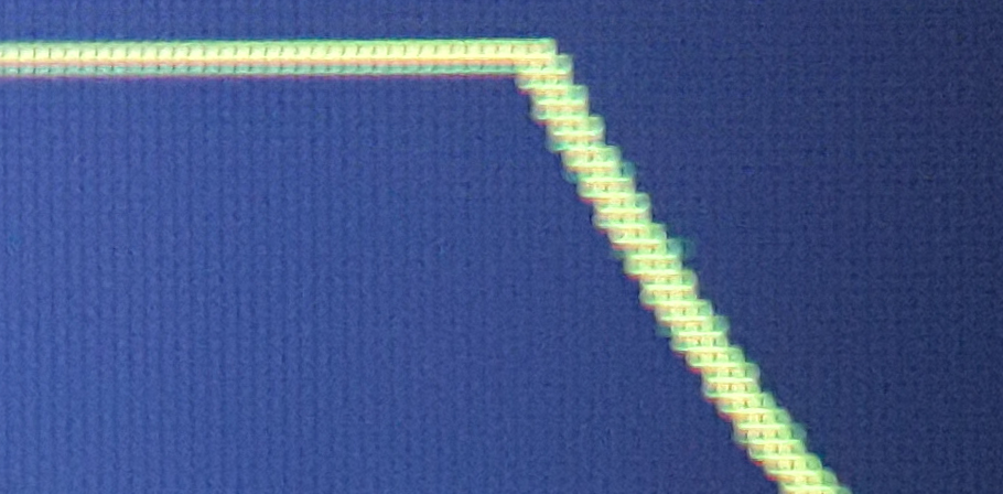
You can see the antialias working both in the stable period at the left (the lower row of pixels is a less intense yellow, indicating the relative position of the sample between the two rows), and in the "stepping" in the curved part.

Side scrolling

For a 'scope style right <- left scrolling display, the overlay layer that holds the rendered summarized pixels is side-scrolled in hardware, with new columns of rendered pixels being placed just beyond the visible area while the original samples are updated on the LCD. At the start of each new frame update, the horizontal offset of the overlay is updated in hardware to include the latest rendered columns at the right.

Considering we may produce 1000 new columns/sec, but can only update the display at 30fps, we may produce 33 new columns of pixels in each 33ms while the previous frame is being sent to the LCD.

That means we need to allow at least an overlay logical size of (160 + 33 = 193) x 128... for practical reasons that was extended to 256 x 128. So we display part of the logical overlay, a 160 x 128 window which can be offset horizontally inside a 256 x 128 overlay framebuffer.

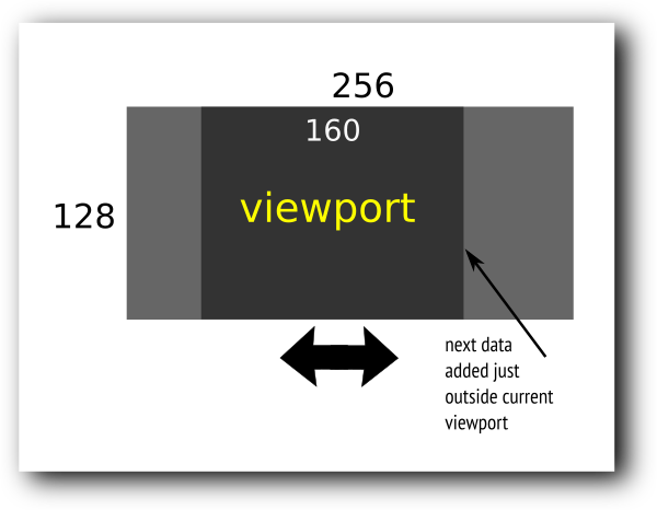
In that way, we can draw new pixels at +160, +161 etc from the offset, while the LCD is being updated with +0..+159 from the offset. Each new frame, we update the offset to be at the last written pixel column - 159.

Hardware wrapping support

Implicit in that scheme though, is that the offset framebuffer must wrap when we scan it out, and we must wrap when we draw ahead of it, from +0xff -> +0 from the current line start.

Consider when we scroll the viewport to actually start scanout at (start of virtual fb line) + 0xb0...

If we just continue linearly reading from the framebuffer after +0xff, we will start to show the pixels from the NEXT line for the remainder of the current line, because +0x100 is the next line.

Therefore in this case halfway along the scanline, whenever we hit +0xff, we must force the FIFOs to restart reading from +0x0 from the start of the current line in the virtual framebuffer.

This is more complex than just reducing the number of address bits incremented, because the data is coming via a rate adaptation FIFO with his own SRAM buffering, which normally would want to read a while line ahead quickly in a few bursts with the Hyperram. So for this overlay channel, the FIFO transaction size is manipulated to be the 2's-compliment of the low 8 bits of the start address: this gives the behaviour of forcing a burst to end after an address 0x....FF while allowing long bursts subsequently.

What we learned this time

The best ways to "compress" a lot of data work by retaining as much of the input data as possible and finding a way to render it
If we decouple the summarizing + rendering action from the acquisition, we get a lot of flexibility to rerender with full sample detail arbitrarily and look at the same data from different ways. That also lets us rerender at full quality into offscreen buffers and display over the network.
Using fractional row mapping, and row accumulators to generate trace intensity information, gives us an extra dimension to drive with sample data. This makes a visible difference in how much information is being rendered and the perceived quality.
Although it's a significant effort, implementing the summarizer in hardware in the FPGA directly connected to the Hyperram allows us to provide both highly zoomed-out (ie, iterating through a large number of samples) and 1:1 (ie, bulk display updates on every frame) summaries for all channels in realtime responsively.